Neuroevolution via Indirect Encodings
Compositional Pattern Producing Networks
CPPNs are a kind of indirect encoding that represents an agent’s neural network as another, smaller neural network. [CPPN2007] Since neural networks act as function-approximators, an agent’s genome is in effect also a function. This neural network approximation of a function will be used to construct an agent’s brain, which is also a neural network.
By representing an agent this way, it is not necessary to encode every connection in the final agent phenotype when performing evolutionary computation to find good solutions. Example
Let’s start with a simple example using epann. Once we construct a population using epann, we will be able to explore a few things:
- How CPPN genomes are similar to the direct encodings of the original NEAT algorithm.
- How a CPPN genome is related to the final agent neural network phenotype.
- How a population of CPPNs reproduce, mutate, and ulimately evolve.
To begin with we initialize a population of agents that each contain a phenotype (an ANN that will directly interact with our task) and a genotype (the CPPN).
from epann.core.population.population import Population

num_agents = 5

pop = Population(num_agents)

for agent in pop.genomes.keys():
    print 'Agent', agent, '-', pop.genomes[agent]
Which outputs:
Agent 0 - <epann.core.population.genome.cppn.CPPN instance at 0x7f4d58219950>
Agent 1 - <epann.core.population.genome.cppn.CPPN instance at 0x7f4d58219ab8>
Agent 2 - <epann.core.population.genome.cppn.CPPN instance at 0x7f4d58219bd8>
Agent 3 - <epann.core.population.genome.cppn.CPPN instance at 0x7f4d58219cf8>
Agent 4 - <epann.core.population.genome.cppn.CPPN instance at 0x7f4d58219e18>
As you can see, each agent is defined as an instance of a CPPN object. Within this object are attributes that define its genotype, which can then be used to construct a phenotype for the agent.
If we set aside the first agent (Agent 0), we will see something familiar. Similar to the original NEAT direct encoding, CPPNs are neural networks that can be described by node and connection genome lists. [ES2012] We can take a look at the CPPN visually first in Figure 4 before we explore how these genomes are related to network structure in the same way we saw in Part 2.
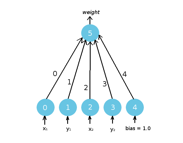
An Initialized CPPN Genotype.
Since an agent’s neural network (Figure 3) and its CPPN (Figure 5) are both networks, we have colored them differently to avoid confusion. The brain of an agent will always have nodes that are colored red or orange, while CPPNs will have blue nodes. CPPNs will have identification numbers on their nodes and connections, while an agent’s brain no longer will.
The Node Genome
From our previous program, we can begin adding genomes to the environment.
agent_index = 0
current_agent = pop.genomes[agent_index]

print current_agent.nodes
Which returns:
{0: {'activation': 'linear', 'type': 'input'}, 1: {'activation': 'linear', 'type': 'input'}, 2: {'activation': 'linear', 'type': 'input'}, 3: {'activation': 'linear', 'type': 'input'}, 4: {'activation': 'linear', 'type': 'input'}, 5: {'activation': 'abs_value', 'type': 'output'}}
Just like we saw before, a CPPN has a node genome that describes the characteristics of its individual nodes. Each key is a node in the genome, and each nested dictionary is that particular node’s attributes. Each of the nodes have an identification number specific to its node genome (written in white in (Figure 5).
For example, Node 5 is an output node (‘type’) with a unique activation function (‘activation’).
(Note: it might seem odd that an output node does not have a more traditional activation function, such as the sigmoid. Neurons in CPPNs can have a variety of activation functions that are selected for their ability to introduce repetition or symmetry, which gives rise to the network’s pattern producing capabilities. More on this distinction later.)
For now, we can at least observe the possible activation functions output nodes can be assigned to:
from epann.core.tools.utils.activations import Activation

acts = Activation()
print acts.tags
Returning:
['x_cubed', 'linear', 'sigmoid', 'ramp', 'gauss', 'abs_value', 'tan_h', 'step', 'ReLU', 'sine']
Nodes within the CPPN (except for the input nodes) can have any of these activation functions. For now, let’s set the activation function to something simple.
# Save the old randomly generated activation function
old_output_act = current_agent.nodes[5]['activation']

# Re-assign the ouput node activation to something simple
current_agent.nodes[5]['activation'] = 'ramp'
We start a generation off with 5 agents that have the same number of input and output nodes. As a result, every agent will have identical node genomes when they are initialized, save the specific activation functions assigned to the output nodes.
# Input nodes
print '\nInput nodes are equivalent across the population when initialized...\n'
for agent in range(num_agents):
    print '\n- Agent', agent
    for node in range(5):
        print '    Node', node, ':', pop.genomes[agent].nodes[node]

# Output nodes
print '\nWhile output nodes differ in their specific activation functions...\n'
for agent in range(num_agents):
    print '\n- Agent', agent
    print '    Node', 5, ':', pop.genomes[agent].nodes[5]
Which returns:
Input nodes are equivalent across the population when initialized...


- Agent 0
    Node 0 : {'activation': 'linear', 'type': 'input'}
    Node 1 : {'activation': 'linear', 'type': 'input'}
    Node 2 : {'activation': 'linear', 'type': 'input'}
    Node 3 : {'activation': 'linear', 'type': 'input'}
    Node 4 : {'activation': 'linear', 'type': 'input'}

- Agent 1
    Node 0 : {'activation': 'linear', 'type': 'input'}
    Node 1 : {'activation': 'linear', 'type': 'input'}
    Node 2 : {'activation': 'linear', 'type': 'input'}
    Node 3 : {'activation': 'linear', 'type': 'input'}
    Node 4 : {'activation': 'linear', 'type': 'input'}

- Agent 2
    Node 0 : {'activation': 'linear', 'type': 'input'}
    Node 1 : {'activation': 'linear', 'type': 'input'}
    Node 2 : {'activation': 'linear', 'type': 'input'}
    Node 3 : {'activation': 'linear', 'type': 'input'}
    Node 4 : {'activation': 'linear', 'type': 'input'}

- Agent 3
    Node 0 : {'activation': 'linear', 'type': 'input'}
    Node 1 : {'activation': 'linear', 'type': 'input'}
    Node 2 : {'activation': 'linear', 'type': 'input'}
    Node 3 : {'activation': 'linear', 'type': 'input'}
    Node 4 : {'activation': 'linear', 'type': 'input'}

- Agent 4
    Node 0 : {'activation': 'linear', 'type': 'input'}
    Node 1 : {'activation': 'linear', 'type': 'input'}
    Node 2 : {'activation': 'linear', 'type': 'input'}
    Node 3 : {'activation': 'linear', 'type': 'input'}
    Node 4 : {'activation': 'linear', 'type': 'input'}

While output nodes differ in their specific activation functions...


- Agent 0
    Node 5 : {'activation': 'ramp', 'type': 'output'}

- Agent 1
    Node 5 : {'activation': 'ReLU', 'type': 'output'}

- Agent 2
    Node 5 : {'activation': 'step', 'type': 'output'}

- Agent 3
    Node 5 : {'activation': 'x_cubed', 'type': 'output'}

- Agent 4
    Node 5 : {'activation': 'x_cubed', 'type': 'output'}
The Connection Genome
The CPPN also has a connection genome that keeps track of the connections between these nodes:
print current_agent.connections
{0: {'enable_bit': 1, 'in_node': 5, 'weight': 1.3157653667504219, 'out_node': 0}, 1: {'enable_bit': 1, 'in_node': 5, 'weight': -0.1669125280086818, 'out_node': 1}, 2: {'enable_bit': 1, 'in_node': 5, 'weight': -0.3487183711861378, 'out_node': 2}, 3: {'enable_bit': 1, 'in_node': 5, 'weight': -1.5476773857272677, 'out_node': 3}, 4: {'enable_bit': 1, 'in_node': 5, 'weight': 0.31068179560931486, 'out_node': 4}}
Just like any neural network you are accustomed to seeing, a CPPN is composed of an input layer (Nodes 0-4) and an output layer (with a single output node, Node 5).
Each agent begins with 6 total nodes which are fully connected, making 5 initial weights. Although agents in the population are structurally identical (they have the same number of initial nodes in their CPPN), the weights of these connections will not be the same for each agent. Similar to before, each connection has an innovation number that identifies it.
Let’s compare a single connection across the population - Connection 0, between Node 0 and Node 5 to show this fact:
print 'Connection weights are randomly initialized across the population for the same connection...\n'
for agent in range(num_agents):
    print '\n- Agent', agent
    print '    Connection', 0, ':', pop.genomes[agent].connections[0]
Gives us:
Connection weights are randomly initialized across the population for the same connection...


- Agent 0
    Connection 0 : {'enable_bit': 1, 'in_node': 5, 'weight': 1.3157653667504219, 'out_node': 0}

- Agent 1
    Connection 0 : {'enable_bit': 1, 'in_node': 5, 'weight': -1.460571493663236, 'out_node': 0}

- Agent 2
    Connection 0 : {'enable_bit': 1, 'in_node': 5, 'weight': 0.4822892299948137, 'out_node': 0}

- Agent 3
    Connection 0 : {'enable_bit': 1, 'in_node': 5, 'weight': 2.042117498128114, 'out_node': 0}

- Agent 4
    Connection 0 : {'enable_bit': 1, 'in_node': 5, 'weight': -1.2561727328710062, 'out_node': 0}
We can verify that Connection 0, which has the innovation number 0 in both the connection genome and in our visualization in Figure 5, describes a connection between Node 0 and Node 5. These landing points are intuitively labeled within the gene: Connection 0 goes out from Node 0 (‘out_node’), and terminates into Node 5 (‘in_node’).
You can go over the connection genome for Agent 0 and compare it to Figure 5 to verify that the rest of the connections share this convention.
for connection in current_agent.connections.keys():
    print 'Innovation #:', connection, '-', current_agent.connections[connection]
Gives us:
Innovation #: 0 - {'enable_bit': 1, 'in_node': 5, 'weight': 1.3157653667504219, 'out_node': 0}
Innovation #: 1 - {'enable_bit': 1, 'in_node': 5, 'weight': -0.1669125280086818, 'out_node': 1}
Innovation #: 2 - {'enable_bit': 1, 'in_node': 5, 'weight': -0.3487183711861378, 'out_node': 2}
Innovation #: 3 - {'enable_bit': 1, 'in_node': 5, 'weight': -1.5476773857272677, 'out_node': 3}
Innovation #: 4 - {'enable_bit': 1, 'in_node': 5, 'weight': 0.31068179560931486, 'out_node': 4}
Just like before, the connection genome has attributes that define the ‘weight’ and ‘enable_bit’ for each connection.
The relationship between an agent’s neural network and a CPPN should still be relatively unclear at this point, and that’s because we’re missing an important component that links the two together.
What are the inputs to a CPPN? The outputs?
A CPPN can act as a mapping by evaluating potential connections in the final phenotype, and the component we are missing in order to accomplish this is something called the substrate: a two-dimensional coordinate space that defines the locations of neurons in the agent’s brain.
The Substrate: Mapping Genotype to Phenotype
An important starting point when thinking about our CPPN abstraction is that we are going to treat our final agent neural network, the brain that will actually be interacting with the task we are interested in, as something that exists in a two-dimensional coordinate space. As a consequence of constructing this plane, individual nodes within a CPPN can be defined with coordinates on that plane.
To begin, let’s place the nodes from our minimum agent controller network onto the plane so that we can investigate these properties.
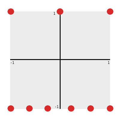
Agent Controller Nodes on a Substrate.
From Figure 6 we can immediately notice a few things:
- The substrate coordinate space is continuous between -1 and +1 in both x and y. (That is, x, y are in [-1, 1].)
- Input nodes can be defined with coordinates that describe their location along the bottom edge of this space: (x_i, -1).
- Output nodes can be defined with coordinates that describe ther location along the top edge of this space: (x_i, +1).
If we assume that within a layer nodes are evenly spaced along the width of the plane, we can initialize their locations as:
import numpy as np

input_locations = [ [ round(xi, 2), -1.0 ] for xi in np.linspace(-1, 1, 6) ]
output_locations = [ [ round(xo, 2), 1.0 ] for xo in np.linspace(-1, 1, 3) ]

print '\nInput locations:\n', input_locations
print '\nOutput locations:\n', output_locations
Where we get:
Input locations:
[[-1.0, -1.0], [-0.6, -1.0], [-0.2, -1.0], [0.2, -1.0], [0.6, -1.0], [1.0, -1.0]]

Output locations:
[[-1.0, 1.0], [0.0, 1.0], [1.0, 1.0]]
The purpose of our CPPN genome is to allow us to more compactly represent an agent’s phenotype with an indirect encoding. The way were are able to do this is by treating a genome as a function of a possible connection in the phenotype. More specifically, A CPPN genome samples a possible connection between two nodes, which are represented within a substrate as a pair of coordinates, and uses them as inputs to the CPPN network. In return, we can receive a property of that connection in the phenotype - for example, the weight of that connection.
| [CPPN2007] | Stanley, Kenneth O. “Compositional pattern producing networks: A novel abstraction of development.” Genetic programming and evolvable machines 8.2 (2007): 131-162.) |
| [ES2012] | Risi, Sebastian, and Kenneth O. Stanley. “An enhanced hypercube-based encoding for evolving the placement, density, and connectivity of neurons.” Artificial life 18.4 (2012): 331-363.) |